NFL: Examining the In-Season Correlation of Defensive Performance

Read more NFL news on BleacherReport.com

NFL: Regression to the Mean, Sample Size, and In-Season Projections

What if I told you that Adrian Peterson isn’t as good as his stats say?

My reasoning is the Curse of the Leading Rusher. You’ve never heard of it before, but it’s an obvious trend. Since 1980, the NFL’s leading rusher has seen his rushing yards fall by 489 yards and his YPC by almost half a yard just one season later. Only six of the 31 leading rushers even increased their rushing yards the following season, and nine had less than 1,000 yards.

Convinced? You shouldn’t be. Their decline is nothing more than regression to the mean and a lack of sample size. Let me explain.

Regression to the Mean

Regression to the mean—also known as the law of averages—is the phenomenon that explains why extreme seasons far from the average (such as a passer rating over 100 or below 70) tend to be closer to the mean the following year.

It’s why we see the leading rusher put up worse numbers the next year, why quarterbacks don’t put up 40 touchdowns in back-to-back years, and, yes, why the Curse of 370 is a myth. Of course, regression to the mean also affects those on the bottom end of the spectrum—Brett Favre won’t throw 22 interceptions again, partly from regression and partly because his past numbers have always been better than last year’s.

Which brings us to the next principle: True score theory. True score theory states that a player’s observed performance is a combination of his true talent level and random error (or “luck,” in layman’s terms). Any time we see a player’s production in a certain time frame (one year, three years, or 10 years, for instance), we expect that his actual true talent level is somewhere in between the observed performance and the league average.

Let’s look at an example. I split all quarterbacks since 1980 into four quartiles based on their fantasy points per attempt, such that the top passers went into one group and the worst went into another. I found the average fantasy points per attempt for each quartile, and then compared that number to the group’s collective next-season value.

The graph below shows this with fantasy points per attempt divided by the average to create an “index value” (where 1.00 is average).

As the blue lines indicate, the quartiles regressed 63 percent to the mean as a whole. In comparison, should Drew Brees regress that much this season, he would have a 50-point drop in fantasy points, which would’ve put him at No. 8 among passers last season. (Of course, that’s assuming no one else would regress.)

I know what you’re thinking. That’s one year of data; of course they’ll decline. Yet regression to the mean even occurs for running backs with three straight 1,000-yard seasons: Those 99 backs averaged over 1,340 yards each of their first three years—with a yards-per-carry rate between 4.33 and 4.36 each year—but they had just 1,161 yards with 4.21 YPC in the next year; almost one-third (32) had less than 1,000 yards to boot.

In other words, those 99 rushers regressed about 45 percent to the mean, which may seem large, but my calculations would’ve predicted a 42 percent regression. That said, their regression was 18 percent less than those of the quarterback example above.

The more sample size we have, the less regression to the mean there is and the more certain we are that observed performance is close to a player’s true talent level.

And that brings us to the next topic.

 

Sample Size, Past Performance, and Mid-season Projections

Most fantasy football players create their own set of rankings usually based on hours of research and trends. So, explain to me why their prognostications should change drastically halfway through the season?

It’s not just Average Joes that do this either. ESPN’s Christopher Harris, for example, ranked Peyton Manning as his No. 2 quarterback in the preseason, but after Week Seven he had dropped Manning all the way down to No. 7.

Manning was 13th in fantasy points (with a quarterback rating just over 80) after seven weeks, but in the final 10 weeks of the season, he was the No. 4 quarterback and had a 105.2 rating, highest among qualifiers.

The moral of the story: Half a season is not enough to warrant a major change in your preseason rankings!

Curious, I went about calculating the change in true talent for players who had a considerable difference in production during the first half of the season compared to their preseason projection. I’m only looking at overachievers, but these numbers also hold for first-half disappointments.

I chose one player at each skill position whose 2009 FEIN projection was equal to a low-end starter in fantasy leagues (Matt Ryan, Larry Johnson, and Eddie Royal) and assumed they were to exceed their preseason projection by 15 percent in the first half (yet with no difference in projected attempts or catches).

Then, based on their projected first-half attempts, I calculated the amount of regression for each player: With 250 first-half pass attempts, for instance, Ryan would be expected to regress about two-thirds back to his preseason forecast in terms of yards per attempt. (I regress to their preseason projection as a shortcut to calculating a whole new set of projections.)

The results indicate that, with 15 percent higher production than expected in the first half of the season, Ryan would only perform 5.4 fantasy points above his preseason projection in the second half, compared to 2.7 for Johnson—including receiving numbers—and 3.4 for Royal.

To further justify the results, the full-season difference between Ryan’s preseason and mid-season projections would not have moved him up a spot in last year’s rankings. (The 10.8-point difference—5.4 doubled—would have increased his 2008 fantasy points from 196 to 206.8, but he would have ranked No. 13 among passers either way.) For Johnson, his outburst would have moved him up just one spot, from 29 to 28, and Royal would have moved two spots to No. 17.

At what point should you adjust your estimate of a player’s true talent? Well, if they overachieved by 15 percent for the first 16 weeks, Ryan’s updated projection would be 16.3 points higher over a full season than his preseason projection (which wouldn’t have moved him up a spot last year), Johnson’s forecast would be 8.4 points higher than expected (a two-spot jump), and Royal’s 9.3-point disparity would have moved him from No. 19 to No. 15.

As a general rule, it takes 21 games for a quarterbacks’ fantasy points to regress 50 percent to their previous projection, as well as 29 to 30 games for a running back and 13 to 14 games for a wide receiver. (The values for quarterbacks and running backs were found assuming there wasn’t a newly calculated projection after 16 games.)

In other words, only for wide receivers should you weigh current-season production more than their preseason projection at any point in the season. That doesn’t mean you should disregard current performance, only that it shouldn’t have as much weight as it usually does when you make trades or waiver-wire pickups.

Remember: If you have a player like Peyton Manning, for whom we have years of stats, then in no way, shape, or form should your opinion of him change after half a season, much less 20 games. Sample size is not your friend, and neither is regression to the mean.

---

This article can be seen at FeinSports.com and FFWritersWithHair.com.

Read more NFL news on BleacherReport.com

NFL: How Breakout and Breakdown Seasons Affect Future Performance

2009 Fantasy Football Projections: Peyton Manning’s Downfall

It’s the middle of August, a time in which many fantasy football owners start to produce their rankings and cheat sheets. Some resort to intuition, while some take an expert’s rankings and tweak them. Others use hours and hours of research to create their rankings.

I’ll use projections.

My FEIN projections (short for Forecasted Evaluative Impartial Numerical projections) aren’t based on intuition or an expert’s rankings or even hours of research. Mine are based on complex algorithms with no human interaction—I input a player’s stats, and out spits their forecast.

 

The Method

Some of you may be wondering how I control for players switching teams or wide receivers losing a top passer, such as Jay Cutler and Brandon Marshall.

I don’t; I only adjust for players who switch conferences. While I could account for this by using air yards, I could only find yards after catch for quarterbacks for the current year, and there was no data for any previous seasons.

The basic steps for any projection system, as well as these, are:

1. Weight each season;
2. Regress each player’s stats to the mean;
3. Adjust for age.

The FEIN projections look at every player-season since 2002. Each stat—passing yards per attempt, interceptions per attempt, etc.—are weighted differently. I looked at all five-year stretches since 1980 and performed tests to see which weight results in the lowest error between actual performance and projected performance.

For instance, completion percentage is weighted as 0.5, meaning 2008 would have a weight of one, 2007 would have a weight of 0.5, and so on down to a minuscule weight of about 0.016 for 2002, whereas interception percentage has a weight of 0.9.

Before I do that, however, I first adjust each player’s stats to a neutral conference. Since 2002, players moving from the AFC to the NFC mid-season or in the offseason have a 2.1 percent increase in passing touchdowns, so I adjust each AFC player’s passing touchdowns down by 1.1 percent (the square root of 2.1 percent, to get them to a neutral conference).

Then, instead of regressing a player’s stats to the league average, I regress it to their height or weight (or BMI). I did further research to follow up my article on height and weight and found that the only stats that are not affected by height or weight are completion percentage, pass yards per attempt, and pass touchdowns per attempt. I regress the first two to the league average, while I regress the third to completion percentage and interception percentage.

What do I mean by that? I found that completion percentage actually predicts future touchdown-to-interception ratio better than that stat itself, and I already saw a relationship between weight and interceptions, so I project first completion and interception percentage, and use that to project touchdowns.

(Side note: The amount I regress each stat to the mean or to height and weight depends on the year-to-year consistency in each stat. What I mean is that completion percentage is more stable than any other passing stat, so a quarterback won’t be regressed as much for completion percentage than interception percentage.)

I then age adjust, adjust for strength of schedule, and then re-adjust for the player’s 2009 conference.

Strength of schedule adjustments admittedly don’t have that much effect; I regress each team’s 2008 defensive stats to the mean (so much so that the Steelers’ 13.9 points allowed per game rises to 18), total up the passing yards per attempt for each team’s 2009 opponents, and then normalize for the league average (such that a team whose opponents allowed a combined 6.7 yards per attempt with a league average of 6.8 YPA would have a YPA factor of 0.985).

I also project rookies as if they were 2008 rookies. Their “2008 stats” are solely based on their projected attempts or receptions. That is, we know that a running back with 200 attempts usually has a higher YPC than one with 100 attempts, or else he wouldn’t have gotten 200 attempts.

So, I looked at all players post-1980 within 20 pass or rush attempts or 10 receptions of each rookie’s projected playing time and found the average stat line of the players in that group. (As expected, the running backs with more attempts had a higher YPC than low-carry backs. Running backs with 188 to 228 attempts—Chris Wells is projected to have 208—averaged one-tenth of a yard more per carry than those with 51 to 91 carries—Glen Coffee is projected to have 71.)

Once I have that, I run the rookies through the same process as everybody else.

 

The Projections

I cheated a little, as projected playing time is an average of ESPN’s, CBS’s, and FFToday’s projected attempts and receptions.

For those without a projection and who played in 2008 (plus Michael Vick), I assigned 20 pass and five rush attempts for quarterbacks, 20 rush attempts and five receptions for running backs, five receptions for tight ends, and 10 receptions for wide receivers.

In the spreadsheet below, overall rank is determined as a player’s VBD, or fantasy points over baseline. My baseline was the number of each position picked in a standard, 192-player draft—24 quarterbacks, 57 running backs, 18 tight ends, and 59 wide receivers.

Some players have “xxx” beside their team and bye week; these players either didn’t play in 2008 or are currently a free agent or retired (in the cases of Vick and Brett Favre).

Without further ado, here are the top-10 in fantasy points at each position. Click here to see the full list.

 

Player	Pos	Comp	Pass Att	Pass Yd	Pass TD	INT
Drew Brees	QB	378	607	4255	33	18
Tom Brady	QB	350	553	4001	29	16
Aaron Rodgers	QB	340	550	3946	29	17
Kurt Warner	QB	354	540	4106	29	16
Philip Rivers	QB	319	513	3772	29	16
Peyton Manning	QB	345	533	3796	27	15
Tony Romo	QB	305	496	3662	28	17
Matt Cassel	QB	316	500	3561	22	13
Jay Cutler	QB	306	495	3615	22	14
Matt Ryan	QB	310	501	3663	23	15
Player	Pos	Rush Att	Rush Yd	Rush TD	Rec	Rec Yd	Rec TD
Maurice Jones-Drew	RB	247	1073	12	60	513	3
Matt Forte	RB	292	1168	10	55	424	5
Adrian L. Peterson	RB	321	1464	12	22	169	2
Michael Turner	RB	334	1438	15	8	48	1
Steven Jackson	RB	291	1203	10	48	401	3
Steve Slaton	RB	277	1241	9	49	385	4
Clinton Portis	RB	315	1330	11	28	213	1
LaDainian Tomlinson	RB	264	1105	12	43	321	2
DeAngelo Williams	RB	271	1235	13	22	139	1
Chris Johnson	RB	264	1196	9	43	312	3
Player	Pos	Rec	Rec Yd	Rec TD
Tony Gonzalez	TE	79	942	7
Antonio Gates	TE	70	839	8
Jason Witten	TE	80	940	6
Dallas Clark	TE	72	802	8
Chris Cooley	TE	73	800	6
Greg Olsen	TE	67	763	6
Zach Miller	TE	62	809	5
Owen Daniels	TE	64	786	5
Kellen Winslow	TE	67	750	5
John Carlson	TE	59	696	6
Player	Pos	Rec	Rec Yd	Rec TD
Larry Fitzgerald	WR	99	1418	10
Calvin Johnson	WR	84	1345	10
Andre Johnson	WR	105	1406	8
Randy Moss	WR	84	1191	11
Reggie Wayne	WR	92	1273	9
Greg Jennings	WR	79	1224	9
Steve Smith	WR	85	1288	7
Roddy White	WR	86	1261	6
Vincent Jackson	WR	71	1140	8
Antonio Bryant	WR	81	1203	7

 

You can download the above spreadsheet into Excel here.

 

The Counter-intuitive Forecasts

The projections aren’t going to be accurate for all 470 players. Here are some of those whose projections seem to go against the grain.

Peyton Manning

Peyton Manning finished in the top four in fantasy points at his position each year from 2002 to 2007, but he slipped to seventh last year. A more telling trend is this: Since his record-breaking 2004 season, both his yards per attempt and passer rating have fallen each year, from a 9.2 YPA and 121.1 rating in 2004 to last year’s 7.2 YPA and 95.0 rating.

The FEIN projections don’t take that into account, but Manning is projected to once again decline in both stats as well as finish sixth among quarterbacks in fantasy points, with this forecast: 64.7 completion percentage, 3796 yards, 27 touchdowns, and 15 interceptions.

Matt Cassel

Matt Cassel went from a career backup to earning more than Tom Brady in just one year, after passing for almost 3,700 yards with 21 touchdowns.

As I mentioned before, the projections don’t take into account any changes of coaching staff, personnel, or teammates, and Cassel is one who would be negatively affected with any adjustments for this.

Last year, 57 percent of Cassel’s passing yards came after the catch, while only 42 percent came after the catch for Kansas City quarterback Tyler Thigpen. Cassel’s raw YPA was a yard higher than Thigpen’s, but his air yards per attempt was less than Chiefs QB.

Since wide receivers have more control over YAC than quarterbacks, it’s likely that Cassel’s projected YPA of 7.1 is optimistic.

Clinton Portis

Clinton Portis’ projection isn’t actually odd at all; it’s just that too many fantasy owners massively underrate him.

Since his rookie season in 2002, Portis has finished outside the the top 10 in fantasy points among RBs just twice—he finished 11th in 2004 and 36th in 2006, when he only played eight games (double his fantasy points and he would finish ninth).

Portis has had one sub-1,200-yard season in his career—2006, when he would’ve finished with 1,000 yards if he played all 16 games. He’s also had two sub-nine-touchdown seasons in his career—2004, the year he finished 11th in fantasy points, and 2006, when he would’ve had 14 if he played all 16 games.

Just when everyone thought he was done, Portis had almost 1,500 yards and nine touchdowns in 2008.

His forecast of 1,330 yards and 11 touchdowns is nothing short of ordinary.

Anquan Boldin

Boldin finished seventh in fantasy points last year despite missing four games due to injury, and he finished the year with 1,038 yards and 11 touchdowns.

Boldin’s projection calls for a YPC rate of 12.4, in line with his past numbers. The seven touchdowns is a major drop from his touchdown percentage the last two years, but receiving touchdowns have a weight of 0.8—which means that 2004, 2005, and 2006 are weighted quite heavily in the forecasts.

We get a career weighted touchdown percentage of 8.9, or 7.2 touchdowns in his 81 projected receptions; that’s slightly less than his exact projection of 7.3 touchdowns.

As well, his No. 17 ranking among wide receivers may be due to his forecasted playing time. Give him 89 receptions, and he ranks No. 12 among wideouts.

Vincent Jackson/Antonio Bryant

Jackson and Bryant were the epitomes of late-round or waiver-wire grabs at the wide receiver position last year. Jackson, selected No. 41 among wideouts in 2008, provided owners with almost 1,110 yards and seven touchdowns. Bryant, taken No. 73, finished No. 8 among receivers, with 83 receptions for 1,248 yards and seven scores; amazingly, Bryant had a higher YPC in 2007 than in 2008.

Fantasy football owners certainly think they’ll both cool off, as Bryant and Jackson are being selected as Nos. 17 and 18 among receivers, respectively.

That doesn’t make sense, even if you discount their projections. Jackson is projected to catch 71 balls in 2009, 12 more than he had in 2008. Thus, he’d need a 25 percent drop in yards and touchdowns per catch (which would give him a new career low in YPC by over a yard) from 2008 to finish as the No. 18 receiver, if only because of his (projected) increase in receptions.

As for Bryant, he’s projected to get 81 catches in 2009. If he even ties his career lows in YPC and touchdown percentage, he’d still end up with 138.3 fantasy points—which would place him right ahead of T.J. Houshmandzadeh, who’s projected to end the season with 138 fantasy points and finish No. 18 among receivers.

I would not suggest you use the bare projections as your cheat sheet. The projections don’t take into account any changes in a player’s surrounding—save for a switch in conferences—and, as such, there’s going to be a lot more inaccuracy in the projections for players switching teams.

Is Matt Hasselbeck the No. 24 quarterback? Maybe he was before T.J. Houshmandzadeh signed with the Seahawks; it’s inevitable that Hasselbeck will outperform his projection, and the same could be said for Matt Ryan with Tony Gonzalez now on the team.

Size Does Matter: How an NFL Player’s Height and Weight Affects Performance

NFL Aging Curves by Position: Rookie QBs, Third-Year WRs, and Age 30 RBs

They say age ain’t nothing but a number.

Twenty-one, 26, 31—what’s the significance? Is age merely just a number, or a baseline for seasonal performance? How can we quantify this?

Aging curves—also called aging patterns or age factors—show the relative performance of a group of players for each age, usually either showing how much (in percentage terms) a statistic improves or declines from one age to the next, or how the production at any age compares to the peak age.

One method used for aging curves it to simply add up the stats for every player at each age and look at the resulting sums. This is flawed, however, for it doesn’t account for the fact that there are many more players at age 24 than at age 34—the difference in yards or touchdowns per attempt won’t offset the disparity in attempts.

You can solve this problem by dividing the sum by the number of players at that age, right? Well, technically, yes, but it’s still not enough.

There’s selective sampling issues using this technique: The players who rack up attempts or receptions at age 21 or 22—their rookie season—are usually the best players, and thus it would appear that a player’s first year or two is one of their best.

At 35 and 36, the only guys left are the ones who have had a very successful first 12 years of their career and, as a whole, are typically better than the average player at age 24 or 25…and thus, it would appear that a player also peaks very late in his career.

The solution is to look only at matched pairs: how each player performs from one year to the next. Instead of comparing the average production at age 24 to age 25, you see how those 24-year-olds do the very next year. This way, you are looking at the same players in back-to-back years; previously, not every player was the same in each sample.

So, if those set of 24-year-olds have a completion percentage of 60 percent, and at age 25 that rises to 63 percent, we are fairly certain that completion percentage is 1.05 times higher (63 divided by 60) at age 25 than at age 24.

But we’re forgetting the most important principle at hand: regression to the mean. Observed production is equal to a player’s true talent, plus luck or random noise. What we are trying to do is to eliminate that noise, because, in general, that luck goes away in the next year. (For instance, running backs with over 1,000 yards since 1980 average 6.23 yards per game less the following year, almost 100 yards in a full season.)

We want to regress a player’s Year X stats, but leave the Year X+1 stats alone. The question is, how much should we regress? I found that a quarterback with 512 attempts, a running back with 439 attempts, and a wide receiver with 45 receptions should have their yards per attempt or reception regressed 50 percent to the mean; there are different rates for completion percentage and the like, and the more attempts or catches a player has, the less he’ll be regressed.

Normalize each player’s two years based on the league average, and we’re finished.

Let’s see how these aging curves stack up for each position.

(Note: My data sample ran from 1980 to 2007. I looked at quarterbacks with 50 attempts, running backs with 30 attempts, and wide receivers with 20 receptions in Year X, no matter how many they had in the next year, because I weighed each of the players’ two years by the minimum number of attempts or catches in the back-to-back years. I excluded any players who switched teams mid-year or in the offseason.)

(Another note: Unless otherwise noted, aging curves shown are “chained” and then divided by the peak level. That is, if yards per attempt falls two percent every year from age 21 to age 30, then age 21 would be given a value of 1.00, age 22 would be 0.98, age 23 would be 0.98 x 0.98, or about 0.96, and so on until 0.834 at age 30. The numbers are then divided by the peak value, 1.00 at age 21. In other words, a player’s yards per attempt would be 83.4 percent of what it is at age 21.)

Quarterbacks

Some might say that a quarterback’s best years are in his mid-20s, pointing to common knowledge and the successes of Daunte Culpepper and even Marc Bulger. Others may bring up Tom Brady, Peyton Manning, Kurt Warner, and Brett Favre as guys who succeeded well into their 30s.

Who’s right?

To see this table in graphical form, click here . (The values are adjusted up or down slightly so the lines won’t collide.)

According to the table, a quarterback’s peak age is 25 for all but one of the stats, with 26 to 28 not far behind. There seems to be a steep, upward trend at the beginning of a quarterback’s career, and a gentler fall from their peak.

Notice how the curves of touchdowns and interceptions are much more extreme compared to completion percentage and yards per attempt, which have a moderate slope.

Not coincidentally, touchdowns and interceptions both have a worse year-to-year correlation than do completion percentage and yards per attempts—in other words, it’s more likely for a player to have abnormal numbers in TDs and INTs than in completions or yards.

A quarterback’s biggest statistical jump is from age 24 to age 25: Take a league-average 24-year-old, and the next year (in 450 attempts), he’ll add 1.6 points to his completion percentage, 67 passing yards, almost two touchdowns, and two-fifths of an interceptions.

That equates to 11 more fantasy points over the course of a season—or roughly the difference between the Nos. 13 and 19 quarterbacks last year.

Last year, Jay Cutler and Aaron Rodgers made the leap from their age-24 to their age-25 seasons. This year? Well, Brady Quinn is the only qualifying player who seems to have at least a part of the starting job locked up; Tyler Thigpen, Kevin Kolb, Drew Stanton, and Troy Smith round out the 25-year-olds.

Quinn showed some promise last year, throwing for 239 yards and two touchdowns in a Week 10 game against Denver (though he followed that up with 14 completions in 36 attempts for 185 yards at Buffalo). Think about picking Quinn late in your fantasy draft, and it could pay off.

Age isn’t the only way to split up quarterbacks; experience matters, too. Although an “experience curve” looks roughly the same as an aging curve, we see that rookie quarterbacks have a major increase in production to their sophomore season. (So much for the sophomore slump.)

Rookies had a four percent increase in completion percentage and yards per attempt, a five percent increase in touchdown percentage, and an eight percent decrease in interception percentage.

Both Matt Ryan and Joe Flacco would see a 10-point increase in fantasy points if those percentages held up. Those 10 points wouldn’t have moved Ryan up in his rank among QBs last year (in terms of fantasy points), but it would have moved Flacco from No. 19 to No. 14, right behind Ryan.

Though Ryan and Flacco may regress to the mean, the increase from their second-year experience may offset that regression.

Running Backs

Few running backs have had the late-career outburst that John Riggins did. Riggins had just one 1,000-yard season through age 28, before a miraculous career turnaround that included four 1,000-yard performances in the next six seasons, not including his 533 yards in eight games in the strike-shortened 1983 season.

From age 22 to age 28, Riggins had 4,655 rushing yards and 28 touchdowns; Riggins had 2,000 more yards and almost 50 more touchdowns from 29 to 36 in the same amount of time (he skipped his age-31 season due to contract disputes).

Let’s see if that trend holds steady for every running back.

Click here for this table in a graph.

The vertical lines on the graph show the values at age 29 and 30. You can clearly see that each stat falls after a running back’s age-29 season, but is the myth that 30-year-old running backs see a dramatic decline any true?

Not really. Age-30 backs lose 1.26 percent off their yards per attempt (.937 divided by .949 in the table above, then subtracted from one) and 2.13 percent of their touchdown rate (.862 divided by .881 and subtracted from one)—a drop of 15 yards and one-fourth of a touchdown for a running back with 1,200 yards and 12 touchdowns.

To put it bluntly, don’t downgrade LaDainian Tomlinson, Brian Westbrook, Jamal Lewis, or Larry Johnson on your running back rankings because they are turning 30. That is, unless you’re afraid of losing less than three fantasy points over the course of a season.

Running backs tend to peak around 22 to 25, specifically at 23 and 24. Fantasy points per attempt seem to have, more or less, a triangular pattern from 21 to 26, but then it ever-so-slightly increases with no set pattern until age 32.

This can most likely be attributed to selective sampling. The longer a running back plays, the more chance for them to peak later in their careers, a la John Riggins.

In addition, if a guy is playing into his early-to-mid 30s, chances are he’s been productive late in his career; if a guy fades away at age 31, with, say, a drop of 500 rushing yards from his previous year, he’s going to get little carries the next year—if he isn’t retired by then.

Running backs have a very short period of increasing performance. Rushing yards per carry increase from 21 to 22, but decrease all but two of the next 11 years; touchdowns per carry increase from 21 to 23 but decrease four of the next five years.

Of course, the largest overall increase for a running back is between his age 22 and 23 seasons, in which his touchdowns go up almost 12 percent and fantasy points increase by 2.7 percent. (Rushing yards, however, decline by about 1.2 percent.)

Steve Slaton, Marshawn Lynch, and Kevin Smith headline this year’s age-23 class. That said, don’t expect a huge breakout: If we adjust each of their 2008 stats based on their expected increase, all of them would have a four- or five-point increase in fantasy points.

Neither Slaton nor Smith would have their rank among running backs in fantasy points changed, while Lynch would move up three spots from No. 15 to No. 12.

Thirty-two-year-old running backs had the biggest decline in production, losing 10 percent of their yards per carry, 16 percent of their touchdowns, and 12 percent of their fantasy points. This year, however, only two New England backs are turning 33: Fred Taylor and Kevin Faulk.

I think it’s safe to say that neither will perform as the top-10 backs you expected in May.

Wide Receivers

Conventional wisdom says that wide receivers have a longer peak than most other positions.

Take one look at the best receivers in the NFL today—Larry Fitzgerald, Randy Moss, Steve Smith, Reggie Wayne, Chad Johnson, to name a few—and it becomes clear that the best wideouts typically have numerous 1,000-yard seasons during their prime.

The numbers, unsurprisingly, back up this notion.

A graph of this data can be found here.

Wide receivers have the latest and longest peak of any skill position. Their best year is at age 27, but ages 24 to 30 aren’t far behind. In fact, in terms of yards per receptions, all but one of those six years (excluding age 27) are within one percent of the peak level.

In other words, a wide receiver with a true talent level of 1,000 yards in a constant number of catches will be within 10 yards of that level all but one year from 24 to 30. (He’d be within 13 yards in that one year.)

This also suggests that a receiver’s breakout or banner year is more reliable in establishing a new talent level compared to those of quarterbacks or running backs. (As well, receiving yards per catch has a higher year-to-year correlation than any passing or rushing stat.)

A receiver’s largest statistical jump unquestionably occurs from age 23 to age 24, when yards per catch increases by 3.2 percent and touchdowns per catch goes up 7.7 percent.

That means a receiver with 1,200 yards and seven touchdowns—who’d rank No. 12 among receivers in fantasy points—would gain almost 40 yards and half a touchdown (seven fantasy points), and would jump four spots to No. 8.

If you didn’t respect him before, it’s hard not to now: Calvin Johnson is turning 24. The second-year receiver finished fifth in the league in receiving yards with 1,331 and tied for first in receiving touchdowns with 12. In addition, Johnson’s average of 17.1 yards per catch was the second-highest of any receiver with 60 catches since 2006.

Applying the aforementioned age adjustments, Johnson gains over 40 yards and one touchdown to his already absurd statistics.

Another receiver turning 24 is Miami’s Ted Ginn Jr. The ninth pick in the 2007 draft, Ginn started 14 games last year and caught 56 balls for 790 yards, 570 more than his rookie season total. Ginn finished No. 33 among receivers in fantasy points last year, but most Web sites rank him around No. 40 for the upcoming season.

Ginn could beat out those prognostications by a large margin if the age-24 increase comes about.

Interestingly, both Johnson and Ginn are also entering their third season. We hear fantasy analysts claiming that receivers break out in their third season, because it takes two to acclimate to the NFL. Is this belief actually a renaming of the age-24 jump?

If so, the increase from a receiver’s second to third season would not be as large as the increase from age 23 to age 24.

And we see just that.

You can find a graph of this data here.

A receiver’s yards and touchdowns both peak in their third year—though that doesn’t necessarily confirm the myth. From their second year to their third, wideouts gain 1.4 percent to their yards and 4.2 percent to their touchdowns, compared to 3.2 and 7.7, respectively, from age 23 to age 24.

It appears as if the third-year wide receiver myth is actually the age-24 increase in disguise.

How NFL Statistics Lead to Wins, Part 3: Salary Cap Efficiency Since 2000

Even an incompetent owner can spend money. It takes an intelligent one, on the other hand, to spend that money efficiently.

In a time when multi-billion-dollar entities are going bankrupt, teams are looking to spend less money on free agent signings and draft picks.

The Tampa Bay Buccaneers, for instance, were $38 million under the cap prior to free agency. They re-signed just six of their 12 free agents and signed just five others, only one of which—running back Derrick Ward—has a chance to start.

In mid-May, Tampa Bay was sitting at $37 million under the cap, and since then the only transaction they’ve made was signing their fifth-round pick, offensive tackle Xavier Fulton, to a $1.93 million deal with a $181,000 signing bonus.

The Eagles weren’t any better: Sitting $29 million under the cap, Philadelphia re-signed one of their five free agents, wide receiver Hank Baskett, to a one-year deal.

Of their other four free-agent signings, only one was signed to a multi-year deal: tackle Stacy Andrews, to a six-year deal reportedly worth $42 million.

Though they traded for tackle Jason Peters and agreed to a six-year, $60 million contract, Philadelphia currently has $30 million in cap space, according to Pro Football Talk.

More than ever, franchises are cutting back on spending, even making moves to simply reach the salary floor.

But, nevertheless, owners and presidents still want the results on the field; they aren’t tanking games at the expense of saving a few million dollars here and there.

No, they aren’t hoping that their lack of expenditures leads to a lack of wins, but merely a cost-efficient approach of getting into the playoffs.

In the final part of this series, we’ll measure which teams are the best at spending as little money as possible to get the results the fans want. Which teams get the most bang for their buck?

I pulled salary data from USA Today’s salary database for every player since 2000. I then totaled up the cap values for each team, as well as the cap value of offense and defense, respectively, and normalized these values based on the year.

(Note that the sum of a team’s player’s cap values are not the same as its total payroll as noted by USA Today—the sum of total salaries is. But total salary, as shown, includes a player’s full signing bonus, so a guy like Ben Roethlisberger, who had a $25 million signing bonus but a cap value of just $7.97 million, has a total salary north of $27 million. As well, the total payroll went over the 2008 salary cap of $116 million for 13 of 32 teams and does not reflect a team’s actual salary.)

Then, using the regression equation in Part 2, I calculated the wins (we’ll call them xWins)—and, like the team salaries, the xWins from just the offense (xOW) and defense (xDW), respectively—for every team since 2000 and compared salary to wins as well as many other stats of note.

Let’s start with individual team seasons. Do the undefeated 2007 New England Patriots come in as the most profitable team of the century?

In the table below, you’ll find the top 10 and bottom 10 teams since 2000 in each of eight different stats. To find cost-efficiency, salary is divided by xWins—the less a team spends per win, the more economical it is.

I have also included efficiency for both sides of the ball as well. For defense, however, xDWins are first added to games played before being divided by defensive salary. Why? Here’s an example:

Team A spends $50 million on defense, and its defense is worth minus-8 wins; their salary-per-win would be minus-$6.25 million.

Team B spends $60 million on defense, which is also worth minus-8 wins; their salary-per-win is minus-$7.5 million. Team C spends $50 million and gets back minus-10 wins from their defense; their salary-per-win is minus-$5 million.

Team A is obviously the most cost-efficient, but their money-per-win is in the middle of the three teams; there’s no way to sort them for A to come out on top.

By adding 16 to each team’s xDWins, Team A’s defense comes out with the lowest salary-per-win of the three teams. (The 16 is a fudge factor, yes, but it’s the only way to come up with correct results using the salary-per-win method.)

All dollar values are in millions of dollars.

Key:
$/W: Salary per xW
O$/W: Offensive salary per xOW
D$/W: Defensive salary per xDW, which is first added to games played
$: Team salary normalized based on year
$ SD: Standard deviation of team’s player’s salaries, adjusted based on team’s average salary; a lower number means a team spread the wealth of their salary between its players
xW: Wins based on the regression equation in Part 2
xOWAA: Wins based on offensive stats only, above the average for that year
xDWAA: Wins based on defensive stats only, above the average for that year

 
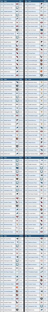
The 2001 49ers had the seventh-lowest team salary since 2000, but their 12.2 xW earned them the top spot among the most economical team of the decade.

Their quarterback, Jeff Garcia, had a cap value of $566,666 yet was elected to the Pro Bowl with a 94.8 passer rating.

Center Jeremy Newberry earned a Pro Bowl berth despite a salary less than $600,000, and safety Zack Bronson had seven interceptions and a salary of $498,000.

Three teams from this past year top the list for the most profitable offenses. The Falcons paid just over $8 million for Matt Ryan, Michael Turner, and Roddy White, two of whom went to the Pro Bowl, and the other of whom (Ryan) had an 87.7 passer rating in his rookie season. Atlanta paid $32 million for 11.9 offensive wins.

Miami’s profit came from its high-paid players: Ronnie Brown was elected to the Pro Bowl after 786 total yards and nine touchdowns in his first 10 games; Chad Pennington was paid $4 million, and his 97.4 passer rating was second in the league; and left tackle Jake Long reached the Pro Bowl in his rookie season. The Dolphins paid $35 million for 12 offensive wins.

Denver would have ranked much higher if not for millions spent on backups. Its highest-paid offensive player—tight end Daniel Graham—caught 32 passes and was second on the depth chart to Tony Scheffler, who earned $3.5 million less than Graham.

Their second-highest-paid player was center Tom Nalen, who missed the entire 2008 season with a torn bicep and eventually retired because of the injury. And their Pro Bowl quarterback, Jay Cutler, was actually paid less than backup Patrick Ramsey, who had three attempts last year.

Without those three, their salary-per-xOW drops below $2 million.

Perhaps the biggest surprise on these lists is that the 2—14 2006 Oakland Raiders had the second most cost-efficient defense—until you remember that their defense was actually pretty decent. (Their 10.5 points scored per game, however, was the fifth-lowest since 1980.)

The Raiders were fifth in the league in yards allowed per play, third in adjusted net passing yards per attempt (and seventh in opponent passer rating), and 13th in rushing yards per attempt. Their defense was above average in xDW, and only the 2004 Indianapolis Colts spent less on defense than the Raiders.

Five Colts teams make the top 10 for standard deviation of player salaries. The ‘03 Colts, who lead the list, spent $15 million on Peyton Manning, $7.7 million on Marvin Harrison, and over a million on 10 others, including $5.4 million on defensive end Chad Bratzke, who ended up starting just three games with three sacks in what was the final year of his career. They also started five rookies, who had an average salary under $500,000.

Based on pure xOW, the ‘04 Colts had the best offense of the last nine years, with the ‘07 Patriots at No. 2. But after adjusting for league average, the Greatest Show on Turf moniker proves correct—the 2000 St. Louis Rams’ offense jumps to the top.

The ‘00 Rams scored what was at the time the third-most points in a season (540), and had the most passing yards, passing touchdowns, and rushing touchdowns—and the second-highest rushing yards per attempt—in the league that year.

Running back Marshall Faulk had over 2,000 yards from scrimmage for the third straight year (he’d accomplish the feat again in ‘01 as well), and set a new NFL record with 26 total touchdowns despite missing two games. His 81 receptions remarkably placed him just third on the Rams.

Kurt Warner had over 300 yards in each of the first six games of the season (he was on pace for over 6,000) and had 17 touchdowns in that stretch, before a broken hand cost him five games. Backup Trent Green took over and had three more 300-yard games. Warner and Green combined for over 5,492 yards, the highest in NFL history.

Interestingly, only one of the top—10 teams in xOWAA won the Super Bowl that same year: the 2006 Colts. Yet the top three teams in xDWAA each won the Super Bowl, as well as the No. 6 team on the list, the ‘03 Patriots. Certainly, this gives some credence to the belief that defense wins championships.

Which brings us to the most economical franchises of the decade. The Patriots have been lauded for their front-office management—but are they really the most cost-efficient? Or do the rival Colts beat them out?

The table below lists each team’s yearly average this decade along with salary efficiency data.

All dollar values are in millions of dollars.

(Want to be able to sort each column? Click here.)

Key:
$/W: Salary per xW
O$/W: Offensive salary per xOW
D$/W: Defensive salary per xDW, which is first added to games played
$/Yr: Team (unadjusted) salary per year
$ SD: Standard deviation of team’s player’s salaries, adjusted based on team’s average salary; a lower number means a team spread the wealth of their salary between its players
xW: Wins based on the regression equation in Part 2
xOWAA: Wins based on offensive stats only, above average (9.21 xOW)
xDWAA: Wins based on defensive stats only, above average (-9.25 xDW)

 
The Colts and Patriots have spent about the same amount of money this decade, yet the Colts have averaged one more xW per year than New England, whose 10 xW per year ranks them fourth in the league.

The Patriots, nevertheless, have won the most games in the nine seasons since 2000 (102, one more than Indianapolis) and rank slightly higher than the Colts in salary per actual win (just $30,000 less).

Meanwhile, the Dolphins rate No. 1 in terms of offensive salary per xOW, despite a below—average offense as shown by their xOWAA; Miami spent $3.78 million less per year than any other team on offense this decade. (Their total money spent on offense was even less than the Texans, who played two less years than Miami.)

The Colts are on top of xOWAA by a large margin, but they rank fifth in offensive salary per xOW because they spent the most money on offense, as well as the largest percent of total salary on offensive players (59.3 percent).

Baltimore’s defense has been worth 2.35 xDWAA, more than half a win above Pittsburgh’s—but the Steelers spent $4 million less than the Ravens each year, earning them a lower salary spent on defense per win.

The Eagles’ average salary has been the highest in the NFL since 2000, $2 M more than the next-highest team. (In fact, they own four of the 10 highest-spending teams this decade, as shown in the first table.)

Their high salaries drop them from second in xW to sixth in $/W; from eighth in xOWAA to 19th in O$/W; and from third in xDWAA to sixth in D$/W.

Philadelphia is also in the bottom 10 in standard deviation of individual salaries, despite having to pay Donovan McNabb, Javon Kearse, and Tra’ Thomas, among others, in the past nine years.

The importance of salary cap efficiency is reflected, simply, in the rankings: The top six teams in money spent per xW have won seven of the nine Super Bowls with two Super Bowl losses this decade, plus a total of 36 playoff appearances and 45 playoff wins.

In baseball, an owner can spend all he wants in order to win a World Series. With a salary cap and penalties for going over the cap, however, NFL teams must manage their payroll economically in order to stay atop the standings at the end of the season, like the Colts, Patriots, or Steelers.

The Effects of the Officials in Super Bowl XL Using Win Probabilities

Pop quiz: Who said regarding the referees, “I felt they were cheating us,” and “The way the refs were going, I wouldn’t have trusted them in overtime,” and that they were “[taking] the game away from us”?

If you answered anyone from the Seattle Seahawks, try again. The answer is former Pittsburgh Steelers linebacker Joey Porter, who said that after the officials overturned Troy Polamalu’s fourth-quarter interception against Indianapolis in the AFC Divisional Round.

The NFL must have heard his message.

Three weeks later, the Seahawks were not only facing the Steelers in Super Bowl XL, but also Bill Leavy and the rest of the officiating crew. In the biggest game on the biggest stage, the officials made so many questionable calls that benefited Pittsburgh, all they were missing was a Steelers’ helmet.

Seattle was called for seven penalties for 70 yards, and Pittsburgh was called three times for 20 yards.

Said Seahawks coach Mike Holmgren, “I didn’t know we were going to have to play the guys in the striped shirts as well.” Jason Whitlock wrote about the officials, “Am I the only one who would like to hear them defend their incompetence?” Michael Smith said that the officials were “giving [Pittsburgh] the game.”

By all means, Seattle was robbed of the Super Bowl, or at least a shot of winning.

In order to quantify the effect of the officials on the game, I turned to the win probability calculator on Advanced NFL Stats, which I previously used to figure out when to go for the two-point conversion.

By looking at the win probabilities of Seattle prior to and after each of the seven penalties handed to them, I could see exactly how much the Seahawks’ penalties hurt them.

Before I get to Seattle, I’ll show the effects of Pittsburgh’s three penalties as a baseline. PRE shows the Steelers’ situation before the penalty occurred, and POST shows what happened after the penalty.

Expected points come from the win probability calculator, and end result is the final outcome of the drive in which the penalty occurred.

Pittsburgh’s penalties lost them an average of 2.7 percentage points on their win probability and less than half an expected point.

How does compare to Seattle? A chart showing the seven penalties called on the Seahawks and the change in their win probability is below, with a description of each penalty and its effect below that.

First penalty—first quarter, 5:53 left, offensive holding: After an 18-yard pass to Darrell Jackson, Seattle was called for holding. The Seahawks went from first-and-10 from the PIT 23 to third-and-16 at their 49. They were well in field goal range prior to the holding call, but had to settle for a punt after failing to convert the long third-down try.

Second penalty—first quarter, 2:00 left, offensive pass interference: Darrell Jackson caught a 16-yard pass in the end zone for an apparent touchdown. But the back judge—Bob Waggoner, who is a Pittsburgh native—called a late penalty on Jackson that pushed the Seahawks back to a 1st-and-20 on the PIT 26.

Seattle kicked a field goal, but if the touchdown to Jackson had stood, the Seahawks would have been driving for the game-tying touchdown on their final possession (which ended on an incompletion on 4th-and-7 from the PIT 23 with eight seconds left in the game).

Third penalty—second quarter, 14:44 left, offensive holding: Seattle returned the Steelers’ third punt of the game 34 yards to Pittsburgh’s 46-yard-line, but holding was enforced at the SEA 35.

The Seahawks took possession at their own 25 and ended up punting at the PIT 47 on fourth-and-two. The 29 yards Seattle lost would have put them at Pittsburgh’s 17 with a chip-shot field goal if there had been no penalty.

Fourth penalty—second quarter, 1:46 left, offensive holding: The Seahawks committed a holding penalty on the kickoff return following Pittsburgh’s first touchdown, which lost Seattle only 10 yards.

Though that may not have seemed like a big difference—what with just 1:46 left and the ball on Seattle’s 27 after the penalty—the Seahawks managed to drive down to Pittsburgh’s 36 and missed a 54-yard field goal to end the half.

Without the holding call, the field goal would have been 44 yards; then-kicker Josh Brown has made six percent more 40-yard field goals than 50-yarders in his career.

Fifth penalty—third quarter, 4:37 left, false start: The most insignificant penalty by Seattle, the Seahawks went three-and-out and punted. Still, Seattle had a 13-yard pass play on third-and-15, which would have been a first down if not for the false start penalty.

Sixth penalty—fourth quarter, 12:08 left, offensive holding: This, on the other hand, was huge. After an 18-yard pass to Jerramy Stevens that ended up on the Steelers’ one-yard-line, the officials called tackle Sean Locklear for holding. The play dropped the Seahawks to the PIT 29 facing a first-and-20, and their win probability fell 17 points.

Two plays later, on third-and-18, Matt Hasselbeck was intercepted by Ike Taylor. Seven points came off the board, and the Seahawks ended with a turnover just outside the red zone.

Seventh penalty—fourth quarter, 10:46 left, low block: On the interception return, Hasselbeck was called for a 15-yard low block penalty. The Director of Officiating for the NFL—Mike Pereira—even said that “the call was not correct” and “should not have been made.”

Nevertheless, the Steelers got the ball on their 44-yard-line and scored on an Antwaan Randle El touchdown pass to Hines Ward.

Although the argument could be made that the Steelers would not have attempted such a trick play on their own 42 (the play occurred 15 yards ahead, on the SEA 43), Hines Ward was so far ahead of his defender that he would have run the extra 15 yards to the end zone.

Adding up all of the effects on the score of each penalty—an extra three points for the first penalty, four for the second call, three for the third, none for the fourth or fifth (maybe Brown misses the 44-yarder), seven for the sixth, and none for the last call—the Seahawks effectively lost 17 or 20 points due to penalties alone.

That would have made the final score 27-20 in favor of Seattle.

The Steelers, on the other hand, lost no points from penalties—two false start calls came on the same three-and-out (and we don’t know if Pittsburgh would go another 70 or 80 yards to score a touchdown if there were no false starts called), and they scored a touchdown on the drive in which a pass interference call occurred.

Would the Seahawks have won Super Bowl XL without the detriments of their seven penalties?

It appears so.

NFL Sport Channel Latest

• Just How Far Would You Go?
• Sorry Rex, But It Isn’t Happening
• Super Bowl Predictions: Five Stat-Free Reasons Why the Eagles Will Reach The Super Bowl
• Seahawks Attempt to Turn Corner With Heavy Pursuit of Pete Carroll
• Bill Cowher Unlikely to Coach in 2010